Terrain Analysis in ArcGIS Pro
Terrain analysis involves the study of the Earth's surface features and their effects on various natural and human-made processes. It includes understanding the shape, slope, elevation, and orientation of landforms, as well as the spatial patterns of these features. Terrain analysis is crucial in fields such as hydrology, ecology, urban planning, and disaster management. By analyzing terrain, we can predict water flow, identify suitable locations for construction, manage natural resources, and assess natural hazards like landslides and floods.
ArcGIS Pro provides comprehensive tools for terrain analysis. It allows users to create, visualize, and analyze digital elevation models (DEMs) and other surface data. With ArcGIS Pro, you can derive valuable information about terrain features, perform hydrological modeling, and generate 3D visualizations. The software's robust analytical capabilities make it an indispensable tool for professionals involved in environmental management, urban planning, and engineering.
In this article we will be using the Shuttle Radar Topography Mission's (SRTM) Digital Elevation Model (DEM) 1-arc Second Global. The dataset was downloaded via Earthexplorer (https://earthexplorer.usgs.gov/). This article will cover examples and steps for terrain analysis.
Watershed delineation and analysis is covered in a different article.
The SRTM payload flew aboard the Space Shuttle Endeavour during the STS-99 mission. SRTM collected topographic data over nearly 80% of Earth's land surfaces, creating the first-ever near-global dataset of land elevations.
The SRTM payload consisted of two radar antennas, one located in the shuttle's payload bay and the other installed on the end of a 200-foot mast that extended from the payload bay. Each SRTM radar assembly contained two types of antenna panels: C-band and X-band. C-band radar data were used to create near-global topographic maps of Earth called Digital Elevation Models (DEMs).
Data from the X-band radar was used to create slightly higher resolution DEMs but without the global coverage of the C-band radar. The two radar datasets were combined to create interferogramatic maps of scanned areas. SRTM measurements took place February 11-22, 2000 (https://www.earthdata.nasa.gov/sensors/srtm).
Software requirement(s):
- ArcGIS Pro 3.3.0
Download package here:
Exercise 1: Prepare the DEM for detailed and accurate Terrain Analysis
1. Load DEM Data
- Download and double click on the Terrain_Analysis_Makah.ppkx to open it. Save your project in a meaningful location.
If you look at the Contents pane, you will notice that I am using a Local Scene with 2D and 3 D layers.
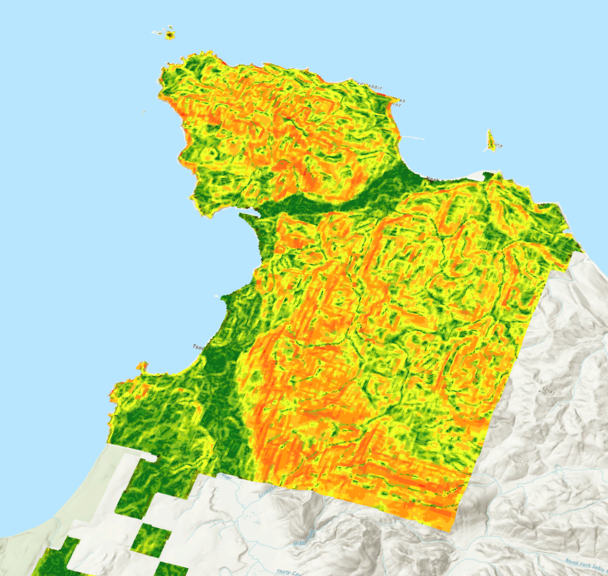
The project has two layers. The SRTM DEM that covers the Makah Nation (WA) and a polygon feature class representing the Makah Nation's boundary (Census Bureau, 2023). The SRTM DEM has been clipped using the Makah's boundary as the Output Extent.

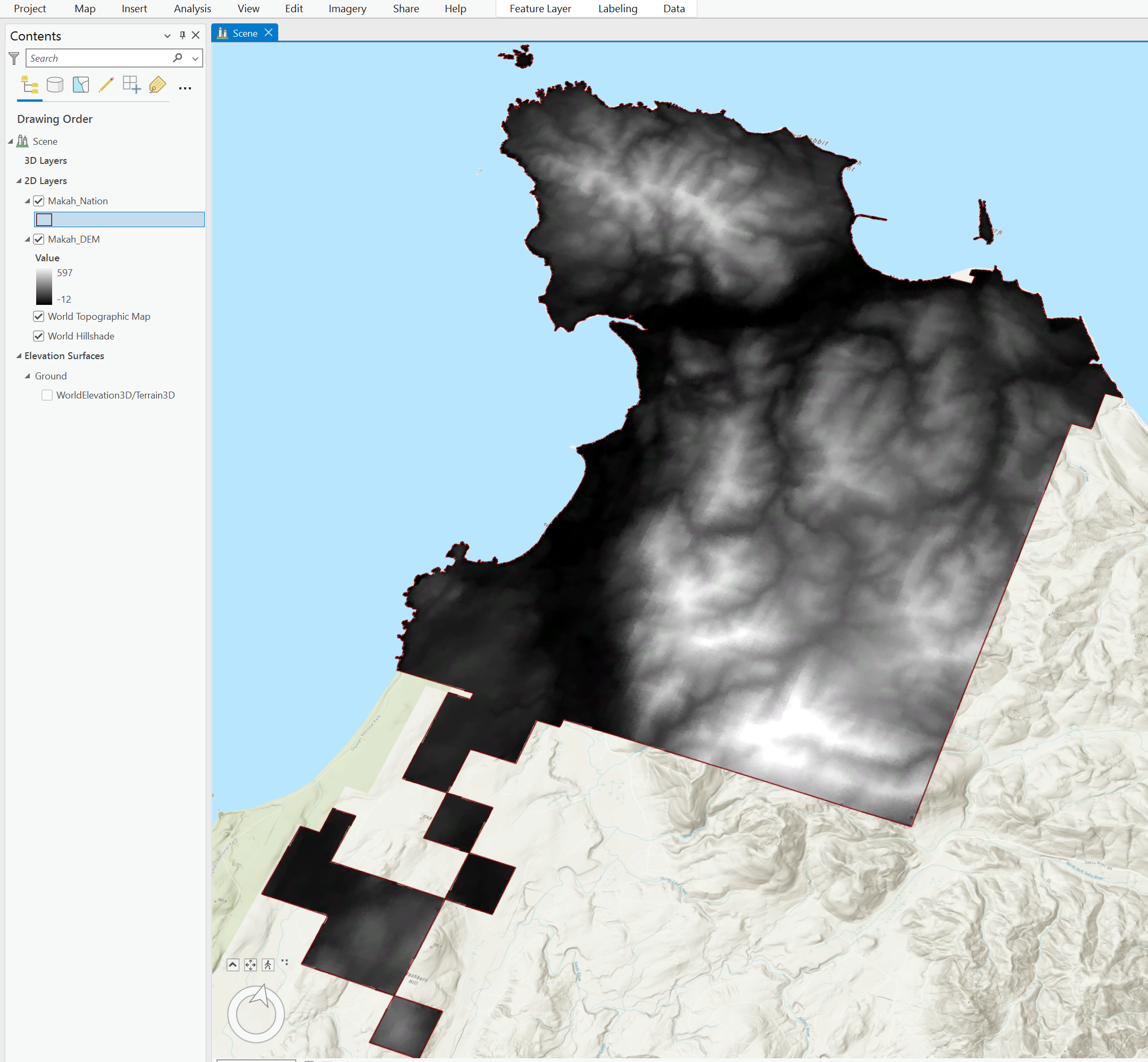
By default, ArcGIS Pro will display the DEM using a black and white color scheme. This is normal and we will improve its visualization.
The SRTM DEM that covers part of the Makah Nation (WA) and Vancouver Island (BC, Canada)
2. Verify the SRTM DEM's Coordinate Systems
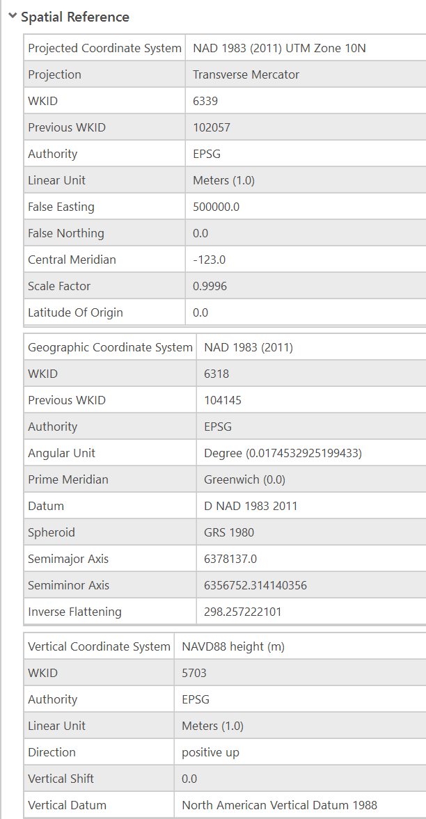
The SRTM DEM is projected in UTM Zone 10N NAD 1983 with Vertical Coordinate System (VCS) of NAVD88. In our example, a gravity-related VCS is necessary. With this in mind, the NAVD88 depth VCS will be sufficient for this project. Specifically, NAVD88 will be more suitable for the data as it is fit for North America and the project location is North American based. All units are in meters.
The VCS NAVD88 (North American Datum of 1988), is a gravity-related height system that provides a standardized reference for elevation data across North America. NAVD88 is based on a mean seal level.
By default, SRTM DEMs have the WGS 1984 Geographic Coordinate System. Projecting SRTM DEMs to an appropriate coordinate system is a crucial step in terrain analysis. It ensures accurate distance and area calculations, consistent spatial resolution, improved performance of geospatial tools, and proper alignment with other datasets.
For DEMs and continuous data, bilinear interpolation or cubic convolution are generally recommended over the nearest neighbor methods. Here's why:
- Nearest Neighbor resampling: Assigns the value of the nearest input cell to the output cell. It is best for categorical data (land use or land cover), where the exact class value needs to be preserved without averaging or altering the values. Not usually used for DEMs because it can introduce a "blocky" or "stair-step" effect in continuous data like DEMs, leading to a loss of detail and precision in the elevation data.
- Bilinear Interpolation: Calculates the output cell value by taking the weighted average of the four nearest input cell values. The weights are based on the distance of the input cells from the output cell. It is most suitable to continuous data, such as elevation, temperature, or rainfall. It smooths the transitions between the cells, preserving the gradient and overall surface continuity. It produces a smoother surface than nearest neighbor and maintain more accurate terrain characteristics.
- Cubic Convolution: Uses the 16 nearest input cell values to calculate the output cell value, applying a cubic function for interpolation. Ideal for continuous data where a high degree of smoothness and detail preservation is required. It generates an even smoother surface than bilinear interpolation, maintaining fine details and gradients more effectively. This method is particularly useful for high-resolution DEMs where preserving subtle terrain is important.
Why choose Bilinear or Cubic Convolution for DEMS?
- Smooth Transitions: Both bilinear interpolation and cubic convolution ensure that transition between elevation values are smooth, preserving the natural gradients of the terrain. This is essential for accurate terrain analysis, such as slope and aspect calculations.
- Minimized Artifacts: These methods minimize the introduction of artifacts that can occur with the nearest neighbor resampling, such as abrupt changes or "stair-stepping" effects that do not reflect the true terrain.
Reasons why reprojected data might not visually appear reprojected
Coordinate System of the Map Frame: the coordinate system of the map frame itself might be different form the coordinate system of your data layers. Ensure that the map frame's coordinate system matches the coordinate system of your reprojected data.
Layer Display Cache: ArcGIS sometimes uses cached displayed data to improve performance, which might not update immediately after reprojecting the data. You may want to clear the cache in the dataset' properties box.
Geographic Transformation: The appropriate transformation might not have been applied and recognized correctly. Check and apply the correct geographic transformation.
Data Extent and Alignment: Differences in data extent and alignment might cause the data to appear misaligned or not reprojected. Verify extent and alignment of your data.
Projection-on-the-fly: ArcGIS Pro projects data on-the-fly to match the map's coordinate system, but the visual appearance might be misleading if there are projection discrepancies. Ensure consistent projection settings.
2. Improving visualization of the DEM
To enhance the visualization of your DEM, applying an effective symbology is essential. I like to use the Elevation #1 color scheme.
- In the Contents pane, right-click on the Makah_DEM.
- Select Symbology.

- In the Symbology window, click on the Color scheme's drop-down menu.
- Enable Show names and select Elevation #1.

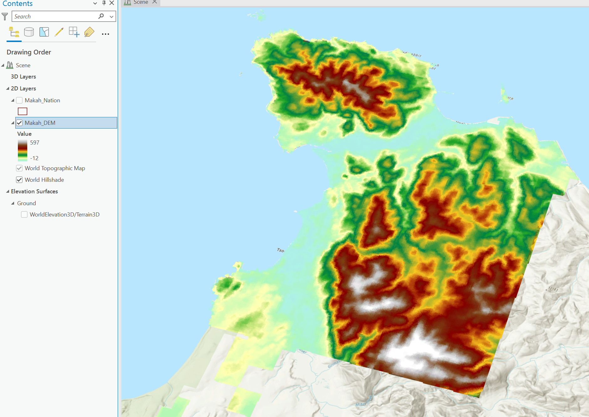
This predefined color ramp provides a gradient from green to brown to white, representing varying elevations effectively. Green typically denotes lower elevations, transitioning to brown for mid-elevations, and white for the highest elevations. This color scheme not only makes it easier to distinguish different elevation levels visually but also highlights the natural terrain features, making them more intuitive to interpret.
Importance of consistent linear and vertical units in Terrain Analysis
Understanding and managing the linear and vertical units of your datasets is crucial for accurate terrain analysis. Linear units refer to the horizontal measurements, such as distances and areas, while vertical units refer to elevation measurements. Some datasets may use meters for linear units and feet for vertical units, or vice versa, which can lead to inconsistencies and errors in calculations if not properly managed. In our example, both the linear and vertical units are in meters, which simplifies the process and ensures consistency. This uniformity allows for straightforward slope and aspect calculations, as well as accurate hydrological modeling and other spatial analyses. Ensuring that both units match eliminates the need for unit conversion and minimizes the risk of errors, leading to more reliable and precise results in your terrain analysis.

Exercise 2: Creating and Analyzing a Hillshade
Hillshade is a valuable tool in terrain analysis that creates a shaded relief representation of a DEM. It simulates the effect of sunlight falling across the terrain, casting shadows to emphasize changes in elevation and the shape of the landscape. By adjusting azimuth and altitude of the light source, different perspectives and times of day can be visualized, highlighting features like ridges, valleys, and slopes. Hillshade is particularly useful for enhancing the visual interpretation of terrain features, making it easier to identify landforms and assess topographic variability.
1. Load Terrain_Analysis project (if necessary)
2. Generate Hillshade
- Go to the Analysis tab and click on Tools.
- In the Geoprocessing pane, search for Hillshade.
- Select the Hillshade tool.
- For Input raster select Makah_DEM.
- For Output raster write Makah_HillS.
- For Azimuth: 315.
An azimuth of 315 degrees means the light source is coming from the northwest direction. Feel free to choose a different azimuth.
- For Altitude: 45
An altitude of 45 degrees indicates the light source is positioned halfway between the horizon and directly overhead. Feel free to choose a different altitude.
- Adjust the Z factor, if necessary, based on your data's vertical exaggeration needs.
The z factor is a scaling factor used in terrain analysis to convert elevation values to the same units as the horizontal distance measurements, ensuring accurate slope and aspect calculations. It is particularly important when the vertical units (elevation) differs from the horizontal units (distance). In our example, since both the linear units and vertical units are in meter, the Z factor is 1, meaning no scaling is necessary. This simplifies the analysis by maintaining consistent units across all dimensions, ensuring precise and straightforward calculations of terrain characteristics.
If the units were different, the Z factor would be used to convert between feet and meters:
- Feet to meters: 1 foot = 0.3048 meters
- Meters to feet: 1 meter = 3.28084 feet
For instance, if the horizontal units are in meters and the vertical units are in feet, the Z factor would be 0.3048. Conversely, if the horizontal units are in feet and the vertical units are in meters, the Z factor would be 3.28084. This conversion ensures that the elevation data is correctly scaled relative to the horizontal measurements, maintaining the integrity of the terrain analysis.
- Model shadows: Enabling the Model shadows option further enhances the realism by accurately simulating shadows cast by terrain features.
Run the tool with or without to see the difference (s).
- Click Run.

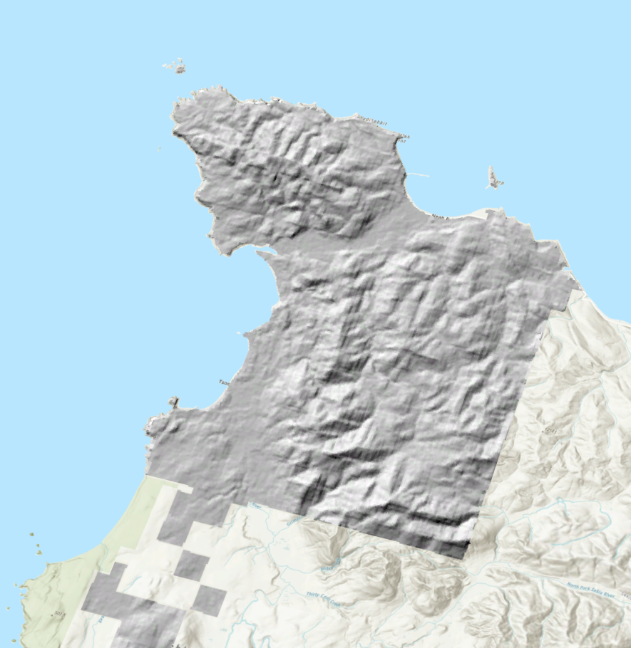
3. Visualize Hillshade
Overlying your DEM on top of the hillshade and adjusting the transparency can significantly enhance the visualization of terrain features. This technique combines the detailed elevation data of the DEM with the shaded relief provided by the hillshade, creating a more dramatic and visually intuitive representation of the landscape. This approach aids in better interpretation and analysis.
- In the Contents pane, make sure that your DEM is above your hillshade.

- Click on the Raster Layer tab and increase your DEM's transparency. Try different settings.


4. Analyze Terrain Features
Observe the shaded relief to identify ridges, valleys, and other terrain features.
Exercise 3: Slope Analysis
Slope is a critical aspect of terrain analysis that measures the steepness or incline of the land's surface. It is calculated as the rate of change in elevation over a specified distance, typically expressed in degrees or as percentage. Slope analysis is essential for various applications, including land use planning, agriculture, and infrastructure development. It helps identifying suitable locations for construction, assessing erosion risk, and planning efficient drainage systems. In agriculture, slope analysis can determine areas prone to soil erosion and inform the design of contour farming practices. Additionally, slope is crucial in hydrological modeling, as it influences water flow direction and speed, impacting flood management and watershed analysis.
1. Load Terrain_Analysis project (if necessary)
2. Calculate Slope
- Go to the Analysis tab and click on Tools.
- In the Geoprocessing pane, search for Slope.
- Select the Slope tool.
- For Input raster select Makah_DEM.
- For Output raster write Slope_Makah.
- For Output Measurement choose Degree or Percent rise.
The choice between degrees or percent rise for measuring slope depends on the specific needs for your analysis and the field of application.
- Degrees are often used in general terrain analysis, providing an angular measurement of slope steepness that is easy to interpret visually.
- Percent rise is preferred in engineering and construction, as it represents the vertical rise over horizontal distance as percentage, making it more intuitive for planning and design purposes.
- For Method choose Planar or Geodesic. In our example, given that the Makah Nation is surrounded by mountains, the geodesic method is the most appropriate choice for slope calculation.
When calculating slope, you can choose between planar and geodesic methods.
- The planar method assumes a flat Earth and is suitable for small areas with minimal distortion.
- The geodesic method accounts for the Earth's curvature, providing more accurate results over large and topographically varied areas. This ensures that the slope calculations reflect the true steepness and variation of the landscape, leading to a more reliable and precise terrain analysis.
- Adjust the Z factor, if necessary, based on your data's vertical exaggeration needs.

- Click Run.

3. Visualize Slope
- Use different color ramps to visualize areas of varying slopes.
4. Analyze Slope
- Identify steep and gentle slopes.
-
Determine suitable areas for construction or potential landslide zones.


When analyzing slopes, you have the flexibility to modify the symbology to better visualize and interpret the results. The symbology settings allow you to classify the slope data using various methods and adjust the number of classes to suit your analysis needs.
Here are some key options for customizing slope symbology:
1 - Classification Methods
- Natural Breaks (Jenks): Identify natural grouping in the data by minimizing the variance within classes and maximizing the variance between classes. This method is ideal for emphasizing significant changes in slope.
- Quantiles: Divide the data into a specified number of classes, with each class containing an equal number of features. This method is useful for evenly distributing the data across classes and highlighting relative differences in slope.
- Equal Interval: Divide the range of slope values into equal-sized intervals. This method is straightforward and easy to interpret, especially useful when you want to show consistent step in slope values across the map.
- Defined Interval: Specify interval size, and the software will automatically create classes based on this interval. This method ensures consistent class widths across the dataset.
- Manual Interval: Manually define the range for each class. This method provides precise control over how slope values are grouped, allowing you to focus on specific slope ranges of interest.
- Geometric Interval: Creates class breaks based on a geometric series, ensuring that each class range has approximately the same number of values and that the change between intervals is consistent. This method is suitable for data with a wide range of values.
- Standard Deviation: Classifies the data based on how much values deviate from the mean. This method is useful for identifying how much a particular slope differs from the average slope.
2 - Adjust the number of classes
You can also change the number of classes to enhance the level of detail in your slope analysis. Increasing the number of classes provides a more granular view of the slope variations. while decreasing the number of classes simplifies the visualization, highlighting broader trends.
Exercise 4: Aspect
Aspect is a crucial element in terrain analysis that refers to the compass direction that a slope faces. It is measured in degrees, with 0 degree indicating north, 90 degrees indicating east, 180 degrees indication south, and 270 degrees indicating west.
Examples Analysis:
Solar Radiation and Microclimate
- Solar Radiation: Aspect significantly influences the amount of solar radiation an area receives. Slopes facing south (in the northern hemisphere) receive more sunlight, making them warmer and drier compared to north-facing slopes, which receive less sunlight and are cooler and moister.
- Microclimate: These differences in solar radiation and temperature create microclimates that affect vegetation patterns, soil moisture, and wildlife habitats. For example, certain plants and animals may prefer warmer south-facing slopes, while other thrive on cooler north-facing slopes.
Soil Moisture and Erosion
- Soil Moisture: Aspect affects soil moisture levels by influencing the amount of sunlight and, consequently, the rate of evaporation and transpiration. North-facing slopes in the northern hemisphere, which receive less direct sunlight, often retain more moisture compared to south-facing slopes. East-facing slopes might receive morning sun and dry out quickly, while west-facing slopes get afternoon sun and retain moisture longer. This can impact the types of vegetation that grow and the overall health of the ecosystem.
- Erosion: The direction a slope faces, and its steepness can significantly impact erosion rates. South-facing slopes, which are drier, may be more prone to erosion due to less vegetation cover and higher evaporation rates. Conversely, north-facing slopes may have more stable soils due to higher moisture retention and denser vegetation, reducing the risk of erosion.
Wildfires
- Fire Behavior: Aspect plays a significant role in wildfire behavior. South-facing slopes, which receive more sunlight, tend to be warmer and drier, creating conditions that can accelerate the spread of wildfires. Conversely, north-facing slopes retain more moisture, potentially slowing fire spread.
- Fuel Availability: The vegetation on different aspects varies, influencing fuel availability for wildfires. South-facing slopes often have more dry vegetation, increasing the fire hazard, while north-facing slopes may have greener, more moisture-rich vegetation.
- Fire Management and Planning: Understanding aspect helps in predicting wildfire risk areas and planning firebreaks and other preventive measures. It aids in developing strategies for controlled burns, firefighting, and post-fire recovery.
Hydrology and Water Management
- Water Flow: Aspect influences the direction of surface water flow and soil moisture distribution. Understanding aspect helps in predicting water runoff patterns and managing erosion.
- Watershed Management: Aspect analysis aids in the design of effective watershed management practices, ensuring optional water conservation and reducing flood risks.
Urban Planning and Construction
- Building Orientation: In urban planning, aspect is considered for building orientation to maximize energy efficiency. Buildings can be positioned to take advantage of natural sunlight for heating and lighting, reducing energy costs.
- Slope Stability: Aspect analysis helps identify areas prone to slope instability or landslide. North-facing slopes may retain more moisture, increasing the risk of landslides.
1. Load Terrain_Analysis_Makah project (if necessary)
2. Calculate Aspect
- Go to the Analysis tab and click on Tools.
- In the Geoprocessing pane, search for Aspect.
- Select the Aspect tool.
- For Input raster select Makah_DEM.
- For Output raster write Aspect_Makah.
- For Method choose Planar or Geodesic. In our example, given that the Makah Nation is surrounded by mountains, enabling the geodesic method is the most appropriate choice for aspect calculation.
- Adjust the Z factor, if necessary, based on your data's vertical exaggeration needs.
- Project geodesic azimuths.
The geodesic azimuth is the angle between the north direction and the direction of the slope, measured along the surface of the Earth, taking into account its curvature. When enabling the option, the tool will adjust the azimuth calculation to account for the Earth's curvature. It ensures that the aspect values are accurate over large and irregular terrain, and that they reflect the true directions of slopes.
- Click Run.


2. Visualize Aspect
You can use the predefined aspect color ramp for a clear visualization or use the symbology to assign colors to different aspect directions (e.g., north, northeast, east, etc.).
3. Analyze Aspect
- Examine the aspect layer to identify the direction of slopes.
- Determine how the aspect might affect environmental factors such as sunlight exposure, vegetation growth, and erosion.
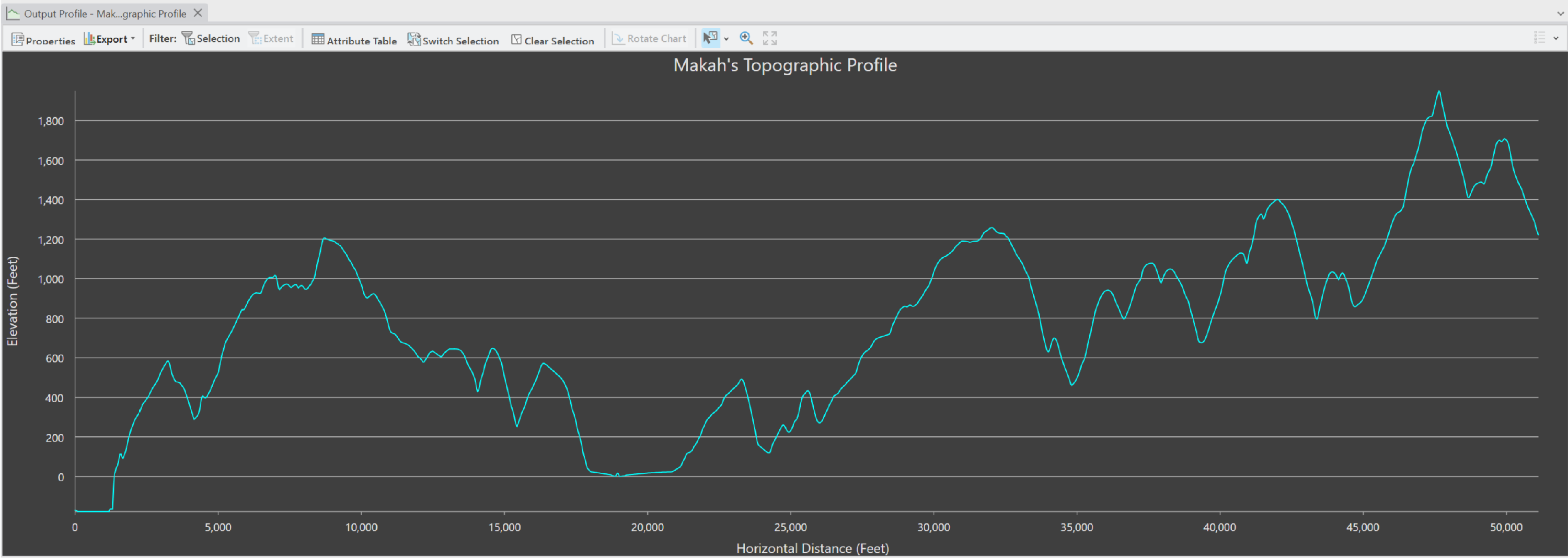
Exercise 5: Topographic profile
A topographic profile is a cross-sectional view that represents the elevation along a specific line across a landscape. It provides a detailed visualization of the terrain's vertical dimension, illustrating the changes in elevation and the slope of the land along a chosen path. By generating and customizing a profile graph, you can gain detailed insights into the vertical dimension of your study area.
Examples Analysis:
Understanding Terrain Features
- Detailed Visualization: A topographic profile helps visualizing the terrain in a way that maps alone cannot, offering a side view of the landscape that highlights elevation changes, slope steepness, and landforms.
- Identification of features: It aids in identifying features such as ridges, valleys, cliffs, and gentle slopes, which are crucial for geological and geomorphological studies.
Planning and Engineering
- Infrastructure Development: Engineers and planners use topographic profiles to design roads, pipelines, and other infrastructures by understanding elevation changes along the proposed routes.
- Construction feasibility: Profiles help assess the feasibility of construction projects by revealing potential changes posed by steep slopes or uneven terrain.
- Environmental and Resource Management
- Watershed Analysis: Topographic profiles are essential for understanding water flow and watershed boundaries, aiding in effective water resource management and flood risk assessment.
- Erosion Control: Profiles help in planning erosion control measures by showing the slope gradients and potential erosion-prone areas.
There are a few methods available. I'll detail two.
FIRST METHOD (from scratch, and if you don't have any predefined line)
1. Load Terrain_Analysis project (if necessary)
2. Create Profile
- Go to the Analysis tab and click on Tools.
- In the Geoprocessing pane, search for Profile.

- In Input Line features: Click on the drop-down menu with the little pencil to create a new feature line in the current DEM to use as input.

- Select Lines.

- On the Makah DEM, draw a line where you would like to create a topographic profile. Right click and select Finish when you are done.

- Profile ID Field: Choose or create a field for unique identifiers (optional). Leave that field empty.
- DEM Resolution: As our DEM resolution is in meters. select the Finest or 10 meters options. This ensures the highest resolution.
- Maximum Sample Distance: Set this value based on your analysis needs (e.g., 10 feet or appropriate distance).
- Maximum Sample Distance Units: Specify the units for the maximum sample distance (e.g., feet).
- Click Run.

- The tool will create an Output Profile in your Contents pane.
- Right click on the Output Profile, select Create Chart and Profile Graph.


3. Customize your Profile
The Properties tab offers various tools to customize and enhance your profile graph.


Axes Tab
Primary and Secondary Axes
- X-Axis (Horizontal): Represents the distance along the profile line. You can customize the scale, interval, and label format.
- Y-Axis (Vertical): Represents the elevation values. Adjust the scale, interval, and label format to suit the elevation range and detail level of your profile.
Tick Marks and Labels
- Customize the appearance of tick marks and labels to improve readability. You can adjust the size, color, and frequency of tick marks.
- Grid Lines:
- Enable or disable grid lines to aid in interpreting the profile. Customize the style and color to fit your visualization needs.
Guides Tab
- Reference Lines: Add horizontal or vertical reference lines to highlight specific elevation levels or distances along the profile. This is useful for comparing different sections of the profile or identifying key elevation thresholds.
- Labels: Add labels to your guides to provide context and additional information. Customize the font, size, and color of the labels to make them clear and informative.
Format Tab
- Background and Borders: Adjust the background color and border style of the profile graph to improve its overall aesthetic and readability. A clear background can make the profile line stand out more prominently.
- Customize chart themes. text elements and symbol elements.
General Tab
- Title and Description: Add a title and description to your profile graph to provide context and make it easier to understand. Customize the font, size, and color of the title and description to match the overall style of your graph.
- Legend: Add and customize a legend to explain the elements in the profile graph. This is particularly useful when comparing multiple profiles or when the profile graph includes additional data layers.

SECOND METHOD
1. Load Terrain_Analysis project (if necessary)
2. Add Elevation Source Layer
The current elevation source layer is set to the WorldElevation3D/Terrain3D. To change it, in the Contents pane right click the Ground surface, Select Add Elevation Source Layer.

Navigate to where Makah_DEM is (Terrain_Analysis_Makah.gdb), select it and click OK.

You have now set the Makah DEM as your elevation surface layer. You can go ahead and remove the other one. Right Click and select Remove.

3. Create the topographic profile
- Go to the Analysis tab.
- In the Workflow groups, click on the Exploratory 3D Analysis icon and select Elevation Profile tool.

- In the Exploratory Analysis window. Change the Distance Units to Meters.

- Now you can click on the map to draw lines. You can draw multiple lines. Double Click to place the last vertex.


- When you hover your mouse over the topographic profile, a highlighted area appears on the profile graph indicating your exact location on the DEM (white dot). This interactive feature allows you to see real-time elevation values and pinpoint specific location on the terrain. It provides immediate feedback and helps you correlate the profile graph with the actual topography of the DEM.

If you need to change your profile line, just click on the blue handles, move it around and it will automatically update.
These exercises provide a foundation for terrain analysis using ArcGIS Pro. By mastering these techniques, you can gain valuable insights into terrain characteristics and their implications for various applications.
We hope that this article has been helpful! If you have any feedback or questions, please feel free to send us an email or connect with us for a chat. The NTGISC team is here to assist you further!
Resource(s):
https://earthexplorer.usgs.gov/
https://www.nist.gov/pml/us-surveyfoot/resources
https://www.washingtontimes.com/news/2019/dec/15/us-ends-survey-foot-use-requires-international-foo/
https://pro.arcgis.com/en/pro-app/latest/help/mapping/properties/pdf/geographic_transformations.pdf
https://pro.arcgis.com/en/pro-app/latest/help/mapping/properties/vertical-datums.htm